Plotting the the difference between NSIDC Extent in 2014 and the stated previous years shows that 2014 is now in 5th place. In recent years July has often seen a levelling in anomalies (average losses), this is happening again in 2014.

The PIOMAS grid box effective thickness map plot is shown below.


Earlier in the melt season Beaufort the the East Siberian Sea (ESS) were significantly thinner than in 2012 and 2013, now thicknesses are comparable due to the stronger spring melts in those regions in PIOMAS. In the Atlantic sector Kara and Barents are significantly thicker this year, the Central and Candian Arctic Archipelago are thicker too.
Plotting volume losses in ten day increments shows how weak volume loss has been in June, it also shows how strong losses were in the previous record year of 2012. Click on the image to enlarge.

Using monthly PIOMAS gridded data the spring volume loss is examined using June minus May volume, the loss within the Arctic Ocean, and within the peripheral seas of the Arctic Ocean is seen to be very muted, even when compared to 2013. In the following graphs that use anomalies, the anomaly is calculated using the 1980 to 1999 average, as usual.

Breaking the above plot down into the regions of the Arctic Ocean, the result is rather a spaghetti graph. But it is clear how the predominance of negative anomalies (greater loss than average) for 2010 to 2012 has failed once again this year. 2014 is a much more mixed year of May to June losses, and like 2013 lacks the large losses in the Central region seen in 2010 to 2012.
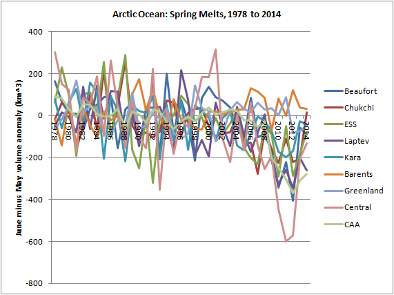
The last three years of spring volume losses show that aside from Laptev, within the Arctic Ocean spring volume loss has been muted when compared with the last two years.

Temperature might seem a reasonable place to look for the cause of this. Certainly the average temperature for May and June north of 70 degN (surface NCEP/NCAR) is low again this year, as last. The following plot is anomaly of temperature, but uses the baseline 1951 to 1980 in line with GISS.

So the reasonable conclusion might seem that the large spring losses of 2010, 2011 and 2012 had nothing to do with ice state and the 2010 volume loss event but were instead caused by weather. However the monthly averages miss detail seen in the daily PIOMAS volume series, daily PIOMAS data has been released now, but I've used up all the time I can spare on this blog post so analysis of that will have to wait.

May 2014 starts off with a strong volume loss, but this fails to continue towards the end of June. Despite this, 2014 looks more like the other post 2010 years than the years before, which suggests sea ice changes following 2010 are still playing a role. That noted, 2009 could be argued to be part of the same pattern. We will have to wait for a few years to see how this develops, whether it continues or not.
In early July compactness (area divided by extent), is notably positive as compared to strongly negative values in recent years. To go back to a similar year one must go all the way back to 2002, 2009 was arguably more neutral than positive. In the following plot compactness for each day from 1 July to 11 July is shown for each year.

This does not argue for greater than average losses during the rest of the season. Mechanistic arguments aside, 2007 and 2012 showed very low compactness at this stage in July, both were followed by new substantial records.
However the open water in Laptev, which seems rather too large to call a polnya, is leading to record low extent in Laptev for 11 July (and for some time before).

Now follows a run down of the regions, starting with all of the PIOMAS domain (all Arctic region), and continuing with the Beaufort, ESS, and Central regions. I use Beaufort, and ESS, as indicative of the Alaskan and Siberian sectors, Kara and Barents are omitted because they virtually melt out by late summer.
All Arctic.
Despite the slow melt this year, PIOMAS data shows 2014 as part of a continuing transition of June thickness from the 2m to 2.9m thickness category down into the 1m to 1.9m grid box effective thickness category. The overall volume increase due to more ice over 3m thick is small when compared to the past declines in such thicker ice, and the transition ongoing around 2m thick.

Similarly the pentad (5 year period) plot of thickness distribution shows that the thickness distribution remains low biassed, and the increased volume for 4m and over thickness is historically small.

Comparing thickness distributions to the other post 2010 years shows how unusual in terms of recent years is the increased volume for grid boxes 4m thick and over. While the peak at around 2m shows that much of the overall volume is more monomodal and around a lower peak of thickness (1.7m) than in 2012 (1.9m), whether or not this difference is significant enough to be considered a reflection of real ice state is debatable.

Finally, here is the progression of thinning of the thickness profile for 2014. As suggested by the previous graphic, this is pretty much normal for recent years, except for the volume at the thicker end of the distribution.

Beaufort Sea.
In 2013 there is seen to have been a large spike of volume in the 2m to 2.9m band, that has not happened this year, indeed volume largely exists in the 1 to 1.9m grid box thickness band. Ice state, as demonstrated by the 1m to 1.9m thickness band plot (red) is clearly in the post 2007 range.

This difference between 2014 and 2013 is clear in the comparison of their thickness profiles, and are part of the post 2007 set, rather than the broader, thicker biassed distribution of pentads for earlier years.

Comparing recent years 2014 is seen to be thinner, and more comparable to 2012 in being monomodal, this suggests a dominance of first year ice subjected to winter thickening. The PIOMAS data suggests that if there has been a large export of MYI into Beaufort, as suggested by the Drift Age Model and ASCAT, then this ice is thinly spread and of low concentration. If PIOMAS is correct we should see melt in terms of extent being vigorous this year, if the MYI is as thick and resistant as some claim it should impede melt. This will be an interesting test. One caveat to my interpretation; I've not had the time to get to grips with PIOMAS sub-grid thickness distributions (gice), it is possible that they hold the signature of a MYI export into Beaufort which is not apparent in grid box effective thickness.

So far this year there has been substantial thinning in Beaufort on PIOMAS.

And so far extent losses in Beaufort have led to extent being below average for the 11 July, and for some time before.

However possible MYI could still cause a slowdown of melt later in the season.
East Siberian Sea (ESS).
Similar to Beaufort the ESS does not show the same increase of thickness in the 2m to 2.9m band as did 2013, rather it suggests part of the continued trend of thinning.

This picture is supported by the long term thickness distributions, 2014 is far more monomodal than 2013 and the 2008 to 2012 average thickness distribution.

Splitting the recent years down supports this picture, the tall thin spike (what I mean by monomodal) indicating a predominance of ethermodynamically thickened first year ice.

Thinning of this first year ice continues from April to June. But be wary of drawing the conclusion that July will only see the same sort of difference from June as June from May and May from April, typically those peaks crash in July (see end of Central Arctic).

In terms of formation of open water, extent is slightly below average, it's even ahead of 2012 which had a broader thicker thickness distribution than this year.

Central Arctic.
2014 has curtailed the promising exponential looking rise in Central Arctic volume from ice 1m to 1.9m, while 2m to 2.9m thickness remains similar to the other post 2010 years, this year the increase in volume from ice over 2m thick is notable.


However, in the context of recent years the increase for volume in ice 4m and thicker is striking.

For completeness, here is the Central Arctic progression of thinning for 2014, not much happening.

But as noted with regards the ESS, don't let the lack of action through to June fool you. As an example of what typically happens in July, here is the progression thinning for the 2013 season in the Central Arctic. And 2013 was a year of poor melt progression.

The shift from the thickness distribution up to June, to July and onwards is marked.
As of 11 July the NSIDC Extent anomaly in 2014 is seen to put 2014 firmly in the post 2010 set. But I still don't think we'll see very large inroads into the Central region this year, unlike 2012.
***
There is one dataset I haven't mentioned, that's Cryosphere Today Area (CT Area). I've not yet had the chance to fully get to grips with Wipneus's extent and area data, so can't comment on whether the following applies to that calculation of area as well. Likewise I've not had a chance to properly compare CT Area and Wipneus Area, my suspicion at present is that I will in due course be dropping CT Area in favour of Wipneus's calculation.
Anyway, CT Area anomalies are currently running level with 2013's at the same time of that year.

On the forum I've previously calculated the following but using late June data, here's an update.
Taking the most recent CT Area data I have access to the 7 days from 4 July to 10 July, I've taken the average CT Area anomaly for this period for each year from 1979 to 2014, call this the early July anomaly. Then I take the 7 day average anomaly centred on 15 September for each year from 1979 to 2013, call this the mid September average anomaly. The early July and mid September anomalies for each year from 1979 to 2013 are used to calculate the late summer summer anomaly drop between early July and mid summer, these are graphed below.

After 2007 these are all negative, in other words CT Area anomalies drop through the summer (losses are greater than average). But even taking into account the whole 1979 to 2013 period the greatest late summer anomaly drop is about -0.7M km^2. So from now until mid September the lowest anomaly drop leads to a CT Area for mid September of 3.1M km^2.
In other words for 2007 or 2012 to be neared in terms of CT Area the losses this summer must not just be above average, they must be so far above average that they exceed the losses for any late summer since 1979. To keep CT Area at 2013 levels by mid September only needs average losses from this point.
4 comments:
Thanks a lot for a great blog post, full of details, Chris.
Thanks Neven,
Probably too many details, but I had to grab the chance of a weekend when I wasn't working overtime.
One detail of interest is that the June thinning in Beaufort is the main contributor to the continued leftward progression of the ~2m thickness peak in your long-term (pentad average) graph for all PIOMAS domains. As Beaufort is where a good part of the 2013 increase in MYI has migrated, its fate in the remaining 2014 melt season seems to weigh heavily on the thickness distributions in coming years.
Iceman,
Yes, I'm seeing possible parallels with the 2010 volume loss event, which also involved such an export.
In 2010 that volume export led to a persistent region of low concentration ice in Chukchi/ESS, eastern Beaufort. As I replied to Neven yesterday - I don't know if that will happen this year, we'll know more by late August.
Post a Comment