The Fast Transition

In May 2015 I concluded a series of posts with The Slow Transition. It was a risky prognostication but an additional 7 years of data has supported what I said back then: That the transition to a seasonally sea ice free state would be slow, not fast, as some argued. This post is about the period preceding that, and with the further 7 years of data something substantive can be said about that.

The Arctic Ocean's sea-ice has undergone a fast transition from one stable mode to another equally stable mode. Between those modes there was a bifurcation driven by the power of an increase of Open Water Formation Efficiency and Ice Albedo Feedback. That bifurcation happened between 2002 and 2006, with the 2007 stochastic event delivering the coup-de-grace that finalised the bifurcation event.

As explained previously, Open Water Formation Efficiency (OWFE) is a non linear function, the function being September Open Water as a function of April sea-ice thickness.

Fig 1. Idealised OWFE (source). 

In and of itself this is not a non linear system which drives change, it is the combination with Ice-Albedo feedback (IAF) and sea-ice memory that drives the change. IAF being the effect whereby sea ice reflects about 80% of incident sunlight, whereas open ocean absorbs about 80% of incident sunlight. So as sea-ice thins to the point where most of its April thickness falls into the region of around 2m thick the IAF drives further loss of thicker ice and forces the above non linear switch from low OWFE to high OWFE. Memory of the sea ice then switches from being longer term (thicker older ice) to short term (one freeze season + one melt season, thinner first year ice).

So there is every reason to expect a bifurcation between the thick multi-year sea-ice stable state (Regime 1) and the thinner first-year sea-ice stable state (Regime 2). I describe these states as stable because absent changes in climatic forcing they would be able to produce persistent statistics of the ice cover. That forcings are changing is not immediately relevant to the question of state stability.

Regimes 1 and 2 are shown in the graph below (click to enlarge).

Figure 2. Two stable regimes in Arctic Sea-Ice.

Both regimes here are defined as the region bounded by average September extent +/-2 standard deviations (95% statistical coverage). 

Region 1 is actually the region following priming of the sea ice, loss of extent over many decades. "Gridded Monthly Sea Ice Extent and Concentration, 1850 Onward, Version 2", Walsh/Chapman et al is a paper that details a long-term series of sea ice extent and contains the following graphic, which I have modified. The dataset is here, however the csv timeseries is not available so I am unable to extend the analysis using that dataset, I don't have the time to get to grips with the NetCDF gridded data. Note also that the graph below is not directly comparable in magnitude with the NSIDC data used in figure 2.

Figure 3. Long term series with Regimes 1 and 2 sketched in (visual approximations)

However the point remains, under some climatic forcing Regime 1 was changing, but remove that forcing and there is good reason to expect a recovery. Remove the forcing to which Regime 2 is subject and it will be harder for a recovery to regime 1 to take place, because Regime 2 is now the 'other side' of a potential wall defined by OWFE and the IAF. 

As mentioned in my previous post about Bifurcations and Attractors, different datasets will not always reveal bifurcations, even when they are there. I have looked at GISS temperature for 64-44N in the graph below. Source, "Zonal annual means, 1880-present..." Note that I have used 44N to 64N so as to include forcings adjacent to, but outside of, the Arctic Region so as to remove substantial signal from feedbacks on temperature within the Arctic Ocean itself. 

Figure 4, Percent Open Water as a function of GISTemp index.

Here the transition to more open water is clear, between blue and grey (Regimes 1 and 2). However on the controlling index, temperature, there is overlap in the horizontal axis between both regimes. In other words, no bifurcation. However, as I have argued, the forcing (temperature) is not the issue in creating the bifurcation.

So instead, in the graphic below I have plotted Percent Open Water as a function of the ratio of PIOMAS ice volume over 2.5m thick and under 2.5m thick as an index of the transition to a thinner ice pack (hereafter known as thick/thin ratio).

Figure 5, Percent Open Water as a function of the ratio of thin and thick ice volume in PIOMAS.

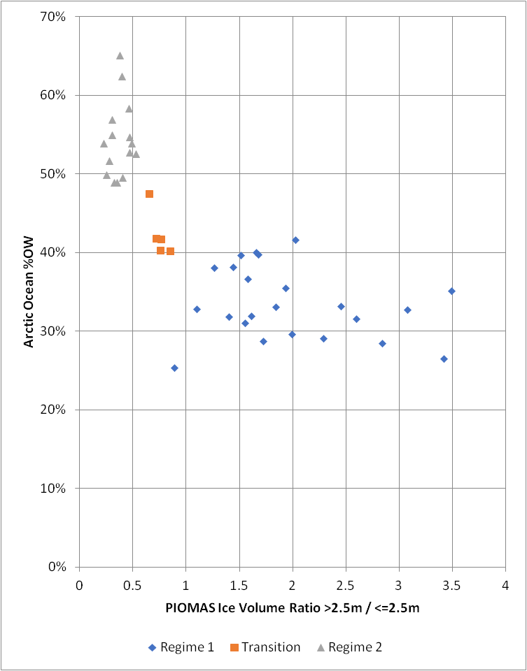
Considering Regime 1, this Regime shows a stable (vertical axis) range of open water despite a massive change in thick/thin volume ratio (horizontal axis). There is one point where the thick/thin ratio is below 1, that was in 1996, supporting the contention that Regime 1 was not condemned to transition to regime 2 because after 1996 the ice recovered, it did not enter the Transition mode. Regime 1 is dominated by thicker ice, and it is the long memory of this thicker ice that allows a substantial trend of loss of volume. However because the thickness remained above the OWFE transition region there was little impact on OWFE, open water formation remained around 30 to 40%.

Then in 2002 the thick/thin ratio declined below 1 and the Transition (bifurcation) occurred (orange points). 2006 was the last year within this period before the weather driven loss event of 2007 which abruptly terminated the Transition and ushered in Regime 2. During the transition open water formation rose from 30 to 40% to 40 to 45%, only with 2007 did it jump to 50 to 60%. Transition was a period dominated by the IAF where volume loss brought thickness of wide areas of the ice pack to the non-linear slope of the OWFE curve. This acted particularly in the BCE region which became a killzone for multi year ice.

In Regime 2, from 2007 the thick/thin ratio was below around 0.5, creating a new grouping of behaviour markedly distinct from either Regime 1 or Transition. By now the pack was dominated by first year ice and became an ice pack with little memory dominated by the thermodynamic growth of young first-year sea-ice. Effectively the loss of sea ice is opposed by the thickness growth feedback leading to a reduced sensitivity to climate forcing as compared to Regime 1.

Figure 6, NSIDC September sea-ice extent was driven by the loss of older thicker ice. 

Most of the extent loss happened between 2002 and 2007.

Any unusual loss of volume in the melt season, such as 2012, was rapidly written over by strong growth of first year ice in the following winter, hence the loss of memory. As a result we are past the fast transition (from Regime 1 to Regime 2) and into the slow transition (to a seasonally ice free state).

Reverting from Regime 2 to Regime 1 faces the potential wall of the slope of OWFE (figure 1) combined with the powerful loss feedback of IAF, together with these being particularly functional in the BCE region. This latter point meaning that for thicker multi-year ice to form (by mechanical deformation) it must somehow survive the BCE Killzone. Ideally the way to explore this dynamic would be in a model like PIOMAS, I lack that facility, but find it hard to see how the above factors do not form a potential wall, which prevents easy transition back to Regime 1. As a result the Transition period from 2002 to 2006 can be viewed as a bifurcation as outlined in my previous post.

Of course, all the above may be just repeating something already in the literature or elsewhere. I just don't have the time or inclination these days to get into reading scientific papers or other blogs.