Open Water Formation Efficiency Part 4

Open Water Formation Efficiency (OWFE) is a measure of the ease with which melt season thinning of sea-ice reveals open water. In March I published a post looking at how this operates from a theoretical perspective. In this post I look at how it operates in practice in various regions of the Arctic Ocean.

Strictly speaking OWFE is the relationship between peak sea-ice thickness in March and the percentage of open water per cm of thinning over the Spring and Summer, originally defined in Holland et al "Future abrupt reductions in the summer Arctic sea ice". Their figure 2b is shown below.

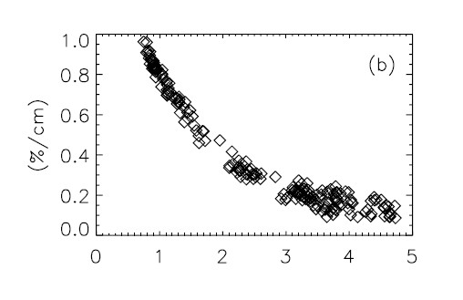
Figure 1. Holland et al 2006 figure 2b, Open Water Formation Efficiency.

However I find the plot form presented in my prior post easier conceptually and more useful. This being produced by a toy model of thinning revealing open water, as described in that prior post.

Figure 2. A plot from a model of open water formation efficiency.

Strictly speaking the above is open water formation, the %/cm is what forms an efficiency, however I'm going to continue the term OWFE for ease as an interchangeable term. The plots below of September percentage open water formation as a function of April sea ice thickness are described as OWFE plots.

So what do the regions reveal?

Figure 3a. OWFE plot for Beaufort Sea.

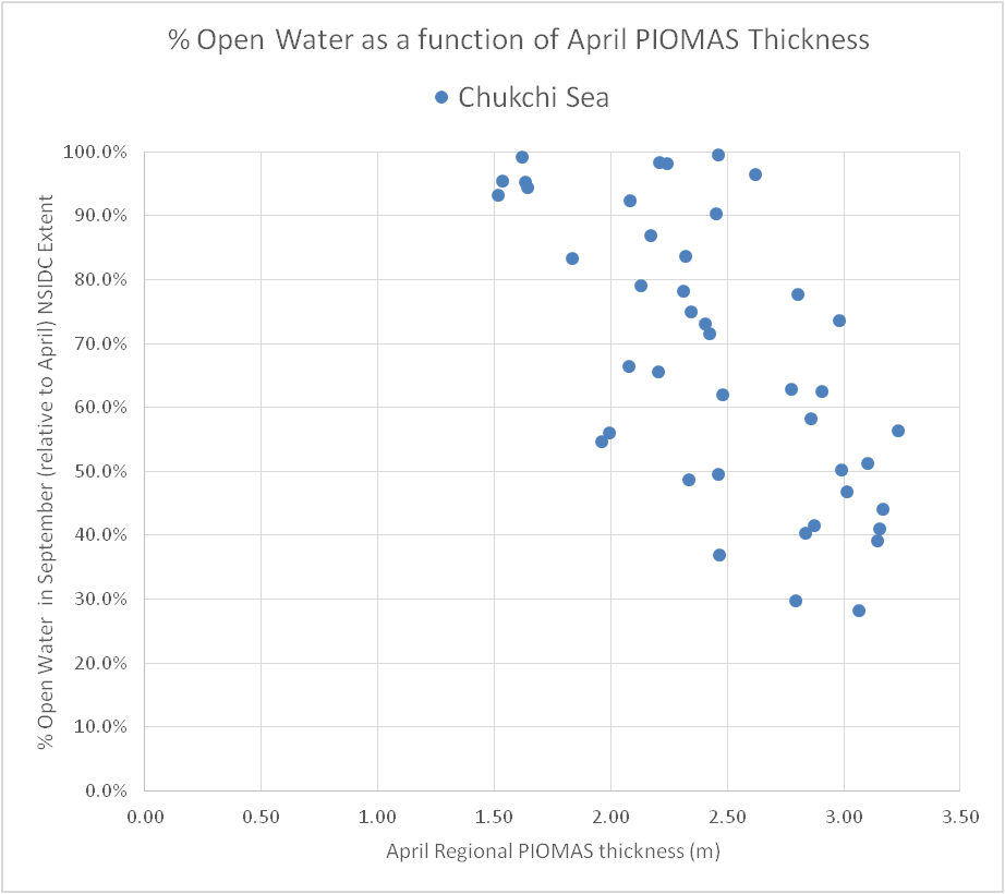
Figure 3b. OWFE plot for Chukchi Sea.

Figure 3c. OWFE plot for East Siberian Sea.

The Beaufort, Chukchi and East Siberian Seas are the BCE region, in a prior post I described how this region has become a 'killzone' for multi-year ice. The above plots show how in each of the seas of the BCE region thinning of ice has increased open water formation, for the net BCE region since 2007 the September open water formation has exceeded 80% in five out of fifteen years.

Figure 3d. OWFE plot for Barents Sea.

The Barents Sea is a proxy for a time in some decades where the Arctic sea-ice is so thin in Winter that melt out to near 100% open water is virtually guaranteed.

Figure 3e. OWFE plot for Central Arctic.

The Central Arctic region shows how far away we are from a virtually sea ice free state. Being at a higher latitude this region will likely need more April thinning because seasonal thinning is likely to be less at higher latitude (something I've not had the chance to check but seems a reasonable assertion.).

Figure 4. Magnitude of role in open water formation for April thickness.

In figure 4 we see a numerical table of correlation and variance (square of correlation) together with the statistical significance limit. So for example in the Beaufort Sea, approaching half of the open water formation is attributed to loss of April thickness and this is statistically significance to the 0.5% level, i.e. 99.5% likelihood that this relationship is due to a real connection, at least 0.5% likely that it is random chance.

From figure 4 it can be seen that for most regions approaching or around half the variance is due to loss of April thickness. The exceptions are Laptev, Barents, and the Central Arctic regions. For Laptev I am not sure why, for Barents and for the Central Arctic this is likely because of the low variation of open water formation (low signal), as seen in figures 3d and 3e above: There is very little vertical variation for the given horizontal variation which results in a low signal of relationship between open water formation and April thickness, in both cases because the regions of activity are away from the steep slope of the relationship around 2m.

Figure 5. OWFE plot for all regions.

In figure 5, above, the same processing of the data as above is carried out for all the regional data amassed into one dataset of April thickness and % open water formation. This is very noisy, so for figure 6 below that data was ordered by order of decreasing open water formation efficiency, and the April thickness was then smoothed with a window centred 7 point running average.

Figure 6, Smoothed data OWFE plot for all regions.

Comparing figure 6 to figure 2 above, the same general form can be seen, something akin to a sigmoid. 

In my previous post I presented just one graphic, a plot of PIOMAS volume from two bands of thickness, with NSIDC September extent superimposed on it.

The match of the volume and September extent is striking, and the extent decline is due to the volume decline mediated by the increase of open water formation efficiency as shown in this post and post 3 of the Open Water Formation Efficiency series. However there is more depth to this. 

In my 2015 post The Slow Transition I wrapped up an extensive series detailing an argument that we had entered a new regime in the Arctic sea-ice, and faced a relatively slow transition to a seasonally sea ice free state. That was controversial in 2015, indeed I drew a lot of flack, but with 6 more years of data it is clear. The implications of this are important and I shall detail these in upcoming posts. Suffice to say for now, up to around the mid 1990s there was an attractor defining a state of September sea ice extent, after 2007 that attractor has gone, a new regime dominated by the thermodynamic growth of sea ice had asserted and we have a new attractor defining a new field of statistics for September extent. Between the states maintained by those two attractors there was a bifurcation and it was not a slow transition at all.

To explain further what I mean, first I must introduce the subtlety and depth of that favourite pastime of cats, knocking things over.