Prediction Update.

On 6 July I made my final prediction for the CT Area minimum, now at 26 August it's worth seeing how that prediction has done, so far.



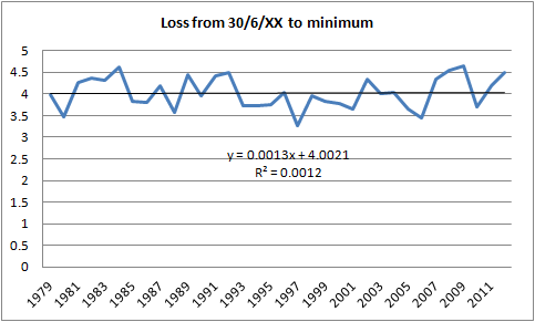
In my CT Area June Status post, link, I made a revised and final prediction for the CT Area index minimum. This was based on the observation of the lack of trend in CT Area losses from 30 June to the annual minimum of CT Area. The plot is for 1979 to 2012, so shows that even in 2012 this behaviour held true.

On 6 July for the Sea Ice Forum July poll I refined that prediction by taking the lower half of the range, to allow for thinner ice than in any year with a similar 30 June CT Area.

As a concession to sea ice state in Laptev to Pole, and thinner ice than in any year that has a minimum between 3.68M and 4.15M km^2, in expectation of a slight fall of anomalies this year I have narrowed the range to the lower half, so my prediction is 3.68M to 3.22M km^2, mid point 3.45M km^2.

This prediction was a massive increase from my previous heuristic prediction of 1.75 to 2M km^2, based on ice state around April. The subsequent cool spring, subdued PIOMAS spring volume loss, and the failure of the summer pattern (the latter two apparent by the end of June) forced a radical re-assessment.

I have previously stated that I expected the prediction to fail by over-shooting, and shortly after 16 July when a fresh wave of melt ponding seemed to occur I was beginning to resign myself to the prediction failing. However from the 24 July a cold weather pattern asserted itself over the ice pack causing a re-freeze and a climb in CT Area anomalies caused by a levelling of CT Area, which is prominent in the plot below, and is highly unusual.

As can be seen from the plot above we are now entering the final stage of the summer, where CT Area levels out, in common with the other (extent) indices at this time of year. From the following graphic it can be appreciated that anomalies tend to be flat from around now until the date of minimum, the only recent year that has seen falling CT Area anomaly over this period was 2012. These flat anomalies indicate that losses, as seen in the seasonal cycle plot above, are around average this close to the minimum. In some years after the flat anomalies, the anomalies fall, this is due to late re-freeze after the minimum has been set.

 

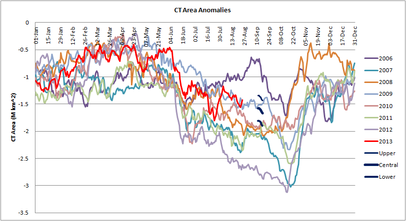
In the above plot the upper, lower, and central figures for the prediction quoted above are presented as anomalies around the typical time of the minimum. It can be seen that only average or slightly below average losses are needed for the close of the season for the prediction to be successful. However it can also be appreciated how much luck has played a role in proceedings to this point; without the cold weather after the 24 August the prediction would by now have been likely to have overshot.

I'll lay my cards on the table: With the likelihood of flat anomalies (average losses) from about now, I am not expecting this prediction to fail.

The lack of trend of 30 June to minimum losses implies negligible impact from the thinning of the ice that has occurred since 1979. So this predictor, having remained reliable in both a year of unprecedented melt (2012) and a subsequent swing to higher amounts of ice, looks very useful indeed. Even if it fails it's hard to see how it can now fail by much. The reverse implication of this is that if this predictor fails massively that alone could be taken as an important indicator of ice state or weather. But I am now certain that 2013 will not see such a massive failure.