The following is figure 3 of Zhang et al 2010. Dotted lines are September volume, solid lines are annual volume. Red up to 2009 is PIOMAS volume using NCEP/NCAR reanalysis for the time up to 2009. Coloured lines after 2010 are projections using random years of NCEP/NCAR reanalysis combined with scenarios A1, B1, A2 & B2.
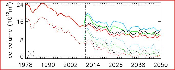
This suggests that at some point the long term loss of volume, upon which I have previously blogged, will reach an inflection with annual average volume ceasing to fall as rapidly, and a long term slower rate of volume loss will establish itself. Zhang et al 2010 state that:
The projected annual mean ice volumes decrease substantially during 2010–2025, with the linear decreasing trends comparable to the hindcast trend over 1978–2009. They decrease at lower rates in later years, particularly over 2030–2050 even as surface air temperature (SAT) continues to increase. One reason is that, although ice melt mainly in summer continues to increase with increasing SAT, thermodynamic ice growth mainly in winter increases too because thinner ice has a higher growth rate [Bitz and Roe, 2004]... ...Another reason is that ice export from the Arctic decreases in the future, just as in 1978–2009 because of reduced ice thickness [Holland et al., 2010].This increase in thermodynamic growth is termed the thickness growth (or growth thickness) feedback, it is a powerful negative feedback noted throughout sea ice scientific literature, especially in modelling based studies. But this is not only a force for the future, it is an ever-present factor in the thermodynamics of sea ice.
In "Inherent sea ice predictability in the rapidly changing Arctic environment of the Community Climate System Model, version 3" (PDF) Holland et al state:
From the 1979–2008 satellite observations, the year-to-year changes in September ice area have a significant negative 1-year lagged autocorrelation (R = -0.59) meaning that an increase in September ice cover is typically followed by a decrease in ice cover the next year. This occurs even with the large downward trend in September sea ice over this time period because the one year reductions in ice are considerably larger than the recovery that often occurs the next year.They explain this as follows:
The observed and simulated negative correlation is likely related to negative feedbacks, such as the fact that thinner ice cover grows more rapidly subject to the same forcing. This fundamental aspect of sea ice thermodynamics gives rise to a negative feedback with a stabilizing influence on sea ice conditions (Bitz and Roe 2004).Note that the above two mentioned papers both refer to Bitz & Roe 2004 "A Mechanism for the High Rate of Sea Ice Thinning in the Arctic Ocean." That paper is, in my opinion, one of the most important papers ever written on sea ice, those interested can find a copy here. But I have discussed that paper in many different posts, here I'm going to approach the same subject of the thickness growth feedback from a slightly different angle.
In my previous post I explained the derivation of the simplest model of sea ice growth. This resulted in the following equation, which is written in pseudo-code form:
Ice thickness = SQRT(InitialThickness^2+(FDD/804.2082)) [Eq 4].
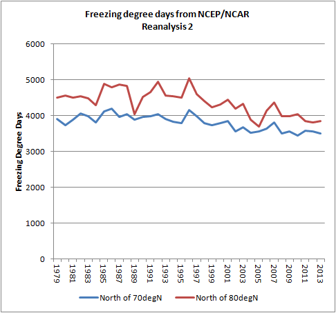
This gives sea ice thickness grown over a freeze season as a function of Freezing Degree Days and Initial Thickness of the sea ice. My calculation of Freezing Degree Days (FDDs) is explained at the end of the last post, but basically FDDs are the sum of the temperatures of days below freezing over autumn and winter. In my calculations I have used -1.8degC as the demarcation of freezing because this is the approximate freezing point of sea water. I have used NCEP/NCAR Reanalysis 2 surface temperatures (T2m) to calculate the FDDs north of 70degN and north of 80degN as an area weighted average from 1 September to 30 April where the stated year is the year in which September falls. Here is the plot showing FDDs for those two regions. EDIT Jan 2016 - only grid cells marked as ocean are used in the calculation.
Using equation 4 we can see how thermodynamic thickening reduces with FDD decline for the case where initial thickness is zero, i.e. sea ice growth from open water.

Because of the square root in equation 4 this declines at an increasing rate, but we are still a long way off dropping April thickness to well below 2m thick, as can be appreciated by the previous plot of FDDs.
So far there is no indication of a collapse in winter cold as indicated by these averaged FDDs for the region north 0f 70degN or 80degN. However this data can be used to plug into equation 4 of my last post (repeated above), and produce average thickening expected from open water (i.e. initial thickness of ice is zero). PIOMAS April thickness is calculated for the regions north of 70degN and north of 80degN for direct comparison to the results using the simple model of sea ice growth for those regions.


The region nearer the pole (north of 80degN) experiences colder winters than does north of 70degN on an area weighted average, so its simulated thermodynamic ice growth is thicker. The PIOMAS average thickness is declining due to loss of thicker multi-year ice and has now reached the levels of thermodynamic growth, but it may well fall below those levels. This can be appreciated in the region north of 70degN, where the PIOMAS average thickness is lower than that calculated using FDDs north of 70degN and the simple model of equation 4. This is to be expected, those who read my previous post will recall I cautioned about the lack of inclusion of snow and ocean heat flux making the model consistently generate thicker ice than a more complete model like PIOMAS.
What is critical here is that equation 4 produces results that are in reasonably good agreement with thickness as generated in PIOMAS, there is a lot of 'whitespace' on the graphs for the model to fail in. And as will be seen, a variation of equation 4 produces a remarkable agreement with PIOMAS data when viewed from the perspective of the thickness growth feedback.
Equation 4 can be modified by subtracting initial ice thickness from it to give ice growth during the period for which FDD is calculated.
Ice Thickening = SQRT(InitialThickness^2+(FDD/804.2082)) - InitialThickness [Eq 5].
This gives an equation that gives ice thickening in terms of FDDs and initial thickness.
Equation 5 can be graphed to give a visual idea of the thickness growth feedback. In the case of the following graph I have chosen an FDD of 4000, reasonable in view of area weighted average FDDs for north of 70degN and north of 80degN.

As can be appreciated from the above, the thinner the ice is in September the more vigorous winter thickening is, this is a simple outcome of thinner ice insulating the atmosphere and ocean worse than thick ice and allowing more heat through the ice, that removal of heat causing sea water to freeze at the underside of the floating sea ice adding to ice thickness. The relationship is strongly non linear due to the square root term in equation 5, an outcome of the basic thermodynamics of ice growth.
Having FDDs north of 70degN I have carried out further calculations using gridded PIOMAS data.
Using 10cm thickness bands the relationship between September PIOMAS sea ice grid box effective thickness and September to April PIOMAS sea ice thickening has been calculated for the whole region north of 70degN. Subsequently this calculation has been repeated for certain groups of regional seas to reveal details. In parallel with that equation 5 has been supplied with the FDDs for each year and the initial thickness in September in 10 cm increments as used in the PIOMAS calculations.
These two parallel sets of calculations result in two 2-dimensional tables of April to September thickening as a function of 60 initial thickness elements (6m / 10cm) and 35 years (1979 to 2013) of FDD data. Jan to April for the year 2014 are in 2015, and that data is not yet available. The average is then taken of the thickening for each initial thickness band across 1979 to 2013.
The results are plotted on the following sets of graphs, PIOMAS is the PIOMAS average thickness growth relationship (blue), Simple Model is the 1979 to 2013 average of the thickness growth relationship obtained from equation 5.
Firstly for the whole region north of 70degN.

OK, to be honest when I first plotted this I was bouncing around with excitement, the agreement between 0.6m and 3.6m (half the total September thickness range used) is far better than I had hoped for. The fall offs below 0.6m and above 3.6m September thickness were a puzzle, but after a bit of thought I had a working guess about each instance, which turned out to be correct. Both snow and ocean heat flux seem to be playing a role here, both were noted in my previous post as deficiencies of the simplest model of sea ice growth.
So how to examine the working guesses? I re-ran the code to generate the PIOMAS thickness growth relationship, this time using the regional codes I have in my data. So here is Beaufort, Chukchi, East Siberian Sea and Laptev, the peripheral seas of the Arctic Ocean not affected by the Atlantic Ocean (which transports significant ocean heat flux to the sea ice).

The blue curve of PIOMAS data is steeper, but the region tends to be warmer over winter than the Central Arctic (lower FDDs), in part because the sun rises earlier there. However the red and blue curves end up tracking well at the top end showing a strong gain in thickening as these seas become mainly seasonal (see my post The Fast Transition).
Now for the regions that make or break the argument. The lower end disagreement between PIOMAS and the Simple Model derived calculations is not visible in the above graph of the peripheral seas that are not affected by the Atlantic. So what of the Atlantic affected regions, Kara, Barents and the Greenland Sea?

Here is seen the cause of the disagreement below 0.6m for the whole region north of 70degN. I suspect that this is due to warming from the Atlantic Ocean waters, ocean heat flux is not factored into equations 4 or 5 and should cause thinner ice and less thickening, especially for thinner ice where heat flux due to ocean warming is greatest. There is a lot of thin ice on the Atlantic margins of the ice pack that stays pretty thin all winter, we appear to see that effect here. However also at play is the odd nature of the Greenland Sea, a transit zone with ice continually being drawn in from the Central Arctic and vented out through the Fram Strait, this would also reduce thickening for thinner September ice.

The only thing that remains to be done is to look at the difference between the simple model (using equation 4) and PIOMAS volume gain from September to April.

As is to be expected from the preceding analysis of the modelled ideal thickness growth feedback, in the Simple Model of equation 4 the feedback is rather too vigorous, not being tempered by the ocean heat flux, snow, and possibly Fram Strait export (and other ice dynamics) present in the more complex PIOMAS model. Nonetheless, both show a recent rise, and I think a reasonable conclusion to be drawn is that the increase in September to April volume gain seen in recent years is due to the thickness growth feedback, as seems to be generally assumed.
This conclusion is reinforced when one looks at the Central Arctic. Here the agreement between the Simple Model (using FDDs north of 80degN) and PIOMAS is far more striking, with a substantial increase in Autumn volume gain largely accounted for by the thickness growth feedback. It is the Central Arctic that must see a crash in winter thickness to enable a crash in summer extent or volume.

Note that Central Arctic volume and thickness has declined during the period since 2003 when the increased autumn/winter gains have occurred, but these declines have been from thicker multi year ice, not ice under 3m thick.

So there is a consistent pattern of good agreement between a simple model of the thickness growth feedback and modelled sea ice data from PIOMAS, where the agreement is broken this is explained by factors not directly related to the thickness growth feedback itself. The thickness growth feedback is a strong negative feedback found in models and visible in reality. In complex sea ice models projected into the future this is a major factor in creating a long tail of sea ice persistence and averting a crash.
Statistical fitting of exponential functions that result in a rapid crash to zero does not contain the physics discussed in this post, that they crash to zero is more a result of the choice of function fitted. Conclusions drawn from such curve fitting of an imminent crash of summer sea ice and the start of a fully seasonal ice pack in the Arctic Ocean should be viewed with great scepticism.
NB, the recent uptick of volume is, in my opinion, a result of weather, not the process of growth thickness feedback outlined in this post.
5 comments:
Chris, comparing the last graph - 'April Central Arctic PIOMAS volume in 5 thickness bands' - with the updated 2015 version (http://dosbat.blogspot.com/2015/08/piomas-july-2015.html) indicates an error either in labeling or data.
2014 April Central Arctic PIOMAS volume in 5 thickness bands
2015 April Central Arctic PIOMAS volume in 5 thickness bands
Thanks for keeping an eye on such matters Kevin, but I think it's OK.
The 2015 update graph is titled 'Arctic Ocean' whereas the 2014 graph is titled 'Central Arctic'. The surrounding text and context seem to me to agree with the use of those graphs. But it is early on a Sunday, so let me know if you still disagree.
Chris;
jdallen from the sea ice blog here.
Can you briefly describe how you are summarizing the NCEP/NCAR data to derive your FDD number?
I assume you are breaking it down regionally and accumulating grid values to produce an average temperature, but want to make sure I follow the same methodology to keep consistent with what you've already done.
Aside from what you've done to understand ice growth, I think it may be a useful proxy in helping understand heat flow and retention in the various parts of the basin. I want to tinker a bit with this years numbers in view of how high the DMI anomalies have been, and see how that translates across the rest of the basin(s).
Going to past years, I will try to unravel any relationship changes in heat flow as implied by FDD's has with changes we see both over all and year over year with the ice.
Sorry to multi post - my goal is to see if there is some identifiable signal which may be predictive. A long shot considering the chaos and complexity of the environment - and the fact that the active melt season is when most of the movement of heat takes place in the basin.
A long shot, but the idea piques my curiosity.
Hi Jeff,
Wow, that's digging back... a year ago!
I have NCEP/NCAR Reanalysis 2 as files for each year, containing the surface temperature for each day and each grid box. I go through the files and in each year work out early and late period area weighted sfc temperature. Early is day 1 to day 120, late is day 244 to day 365. Area weighting of temperature is done by:
TemperatureArea = TemperatureArea + (Temperature - 271.35) * GridAreas(Lat) 'sum up the product of temp and area
i.e. temperature is recacalculated as the temperature difference from -1.8degC and this is then multiplied by the grid box area for that temperature. FDD for the Early or Late period is then calculated as:
FDD = FDD + TemperatureArea / TotalArea 'area weighted average of FDD north of 70degN over ocean
Oh and a step I left out - I use the ocean mask for the gridded data to mask so I only use ocean grid boxes.
And.. the grid is a 192 longitude 94 latitude grid boxes. But so I use the grid boxes north of 70degN I only use the first 11 grid boxes.
Next step to explain is how to work out the grid box areas.
http://www.pmel.noaa.gov/maillists/tmap/ferret_users/fu_2004/msg00023.html
Area of a latitude band
= 2*pi*R^2 |sin(lat1) - sin(lat2)|
So the upper bound of a lat band is Lat1 the lower is Lat2, R is the radius of the earth. I use the polar radius 6,356.75km as my calculation is around the pole and the earth is an oblate spheroid. My calculation gives a -0.45% error from the area of one hemisphere (polar radius is less than equatorial radius), so the method is OK.
Post a Comment