Figure 1, PIOMAS volume anomaly.
It's clear that already by 31 May the trajectory of 2012 is very similar to both 2010 and 2011, and different from years before. The current anomalies are massively lower than for any year before 2010. Using the Cryosphere Today area it is possible to calculate a naive average thickness, calculated thickness. Being the average of the whole of the PIOMAS domain this peaks in June, after the peripheral seas have lost their thin ice but the central Arctic hasn't begun to thin, and reaches a minimum in November due to rapid expansion of thin ice in the early part of the freeze season (October to March).
It is possible to graph the calculated-thickness for the last day of each month, which new PIOMAS monthly run up to. I've used the demarcation of freeze (October to March) and melt (April to September) seasons to separate out the melt season and make the graph legible. It seems fairest to do it this way rather than select some arbitrary set of months.

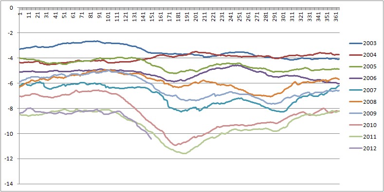
Figure 2, melt season calculated thickness for the last day of each month.
The above figure shows how odd the behaviour of calculated-thickness has been in the months of July, August and September 2010 and 2011. But will we see another unusual continual loss of thickness through the summer, as manifested by the loss of the Roof?
The calculated-thickness anomaly shows that even though it is too early to claim we're following the same trajectory in terms of the above graph, we do seem to be following the same trajectory in terms of calculated-thickness anomaly.
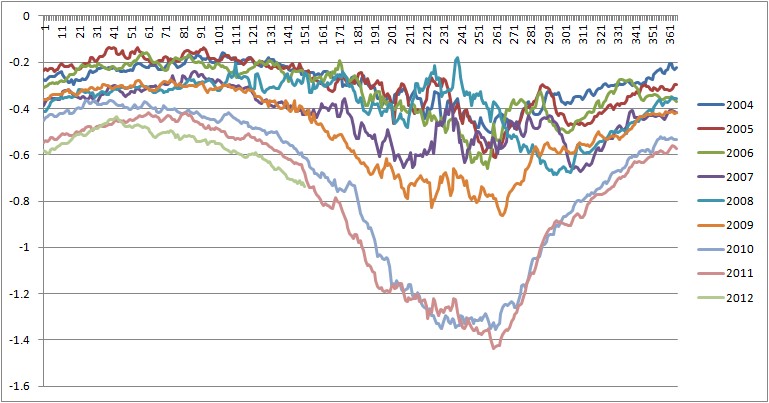
Figure 3, calculated-thickness anomaly for recent period.
Figure 2 shows how odd the behaviour is for the past 34 years, this long term context is lacking in figure 3 above. However the anomaly plots for earlier periods also show that such behaviour is rare.

Figure 4, calculated-thickness anomaly plot for the 1980s.
In both the 1980s and the 1990s there is a year following an unusually low volume anomaly the exhibits a Spring melt leading to a summer volume low. In the 1980s - 1981 leads to 1982, and in the 1990s - 1995 leads to 1996. In both cases the Spring/Summer volume loss starts around day 100 and ends around day 200, but in both cases the anomalies are substantially smaller than in recent years. This behaviour convinces me more that the similarity between 2007, 2009 and 2010/11 is not mere coincidence. Although I can't yet explain the behaviour, it seems to me to be a response to low sea ice volume, one that is being amplified in recent years and I think will very likely repeat again this year.
Despite the significant gaps in my understanding, the behaviour shown in May's data in figure 3 leads me to expect that we will see a repeat of 2010 and 2011 in terms of volume loss. Regarding those gaps in my understanding; this blog will be quiet for at least the rest of this month as I am busy working on new data.
2 comments:
we will see a repeat of 2009 and 2010 in terms of volume loss
You mean 2010 and 2011, right?
Yes I do. Thanks Neven.
Post a Comment