There is a new feature of the Cryosphere Today Area series (CT Area), a June crash in anomalies, this is an important feature, which I suspect is a useful indicator of conditions that prime the ice pack for record melts.
The anomalies for CT Area are shown below. Anomalies are the difference from the long term average seasonal cycle of the ice pack.
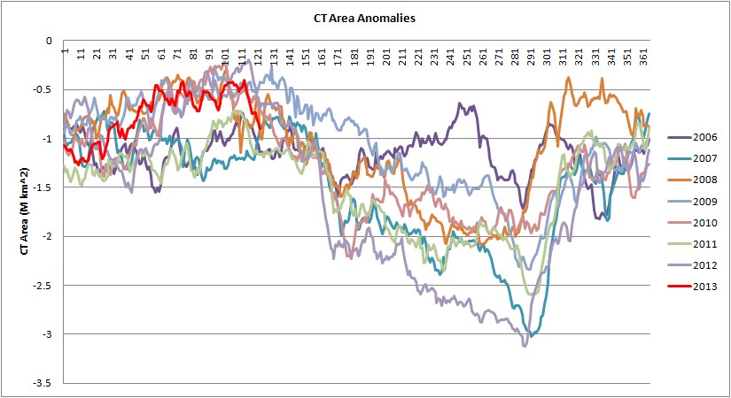
It can be seen that in 2007, 2011 and 2012, there is a rapid drop in anomalies from after the first week in June. These years show a drop, with no recovery, in 2010 there was also a drop but a recovery in anomalies followed. This was because whatever caused the drop, afterwards there was a lesser reduction of area when compared to the long term average. The significance of these years in the longer term context can be appreciated from the earlier post in which I gave CT Area anomalies in graphics from 1980, link.
What is notable about 2007, 2012 and 2007, is that 2007 was a record breaking crash, 2011 was a 'tie' (a new record in some indices but not in others), and in 2012 there was a record breaking crash.
I've previously blogged on research into melt ponds by Rösel & Kaleschke, link. Using MODIS, they find that in 2007, 2010 and 2011, there were high levels of melt pond formation in comparison to other years (2000 to 2011).
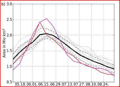
The graphic above is from Rösel & Kaleschke, figure 3b. Along the horizontal axis are dates (18 May, 1 June, 15 June etc), the vertical axis shows area of melt ponding. 2007 (red line) and 2011 (magenta) against the average for 2000 to 2011 (black with one sigma bounds in dashed lines).
Below is a detail from the CT Area anomalies showing the June anomaly crash.
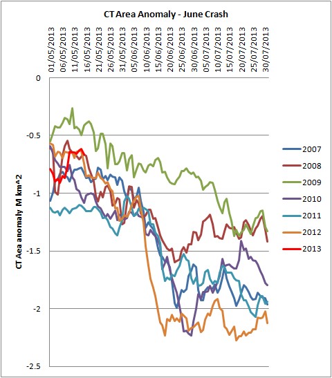
It can be seen that the anomaly crashes are happening around the same time as melt pond fraction is at its greatest. This is exactly the sort of 'contamination' of the measure of sea ice extent/area that the extent indices seek to avoid. In area the area of ice within a grid box is the fraction of ice shown by the satellite sensor, the sensor can pick up melt ponds as open water. In extent any grid box with more than 15% ice is counted as fully ice, so 'contamination' of the data by melt ponds is reduced to near zero giving a conservative measure of the amount of sea ice. However in being conservative important indicators, such as the June crash are not reflected.
Anyway, in 2007 and 2011 Rösel and Kaleschke find record June melt ponding, in the same years there is a crash in June CT Area anomalies. I have been unable to find independent information about melt pond area in 2012 in the context of previous years, but my working assumption is that the size of June CT Area anomaly crash is probably indicative of the area of melt ponding.
However as I have asserted before, the occurrence of June CT Area anomaly crashes post 2010 is supportive of the volume loss of 2010 being a real event, link.
I had thought that the June crash was due to rapid reduction of ice from the periphery of the pack. This is not the case. Using Cryosphere Today's regional breakdowns, link, it is possible to examine the change in anomalies during June 2012. Having the full series broken down into regions would be preferable, but as this is not available I will just have to make do with what I have.
The full decline in anomalies worked out by eye from the graphs is around 1.16M km^2, this is of roughly the same order as the June crash in the orange (2012) plot line in the above graphic. Of this the central Arctic shows a decline of around 0.4M km^2, a substantial fraction of the overall decline and the largest single contributor by far.

So whilst recession of the ice edge in the peripheral seas has a role, in 2012 much of the decline was due to an apparent lowering of concentration in the central Arctic, into which the ice edge had not penetrated by the end of June, i.e. University of Bremen, 1/6/12, 30/6/12.
While the exact mechanism is unclear, what is clear is that whether mainly due to low concentration ice, or melt ponds masquerading as open water, the June crash is associated with September record minima. This makes sense as melt ponds lower albedo, trapping more sunlight and warming the ice, promoting melt, and the same applies to leads between the broken floes of ice typical of summer conditions.
This year we see a record expanse of first year ice, this matters because first year ice is typically flatter than multi-year ice and more prone to developing melt ponds. Also if the ice profile is thinner opening of cracks between floes is more likely to develop open water within the pack, warming the waters within.
I have previously blogged on conditions shown by PIOMAS in March, link, and reflected in both ASCAT and the Drift Age Model (DAM) in December, link. Now DAM data is out up to the end of April.
There are ridged areas and areas of thicker ice within the expanse of first year ice, but it seems to me that the prospects for melt ponding and low concentration across that expanse are substantial this year. I expect a very large June anomaly crash starting in about three weeks. I hesitate to say I expect it to beat the 2012 record June anomaly crash, but I can't think of a logical reason for hesitation.
8 comments:
It's clearest in the Laptev where there was an anomaly drop of something like 200k in the last couple of days of May, which then stopped dead with essentially no further change in area throughout the whole of June. We all saw (and extensively discussed) the "blue ice" appearance of the melt ponding at the time.
http://arctic.atmos.uiuc.edu/cryosphere/IMAGES/recent365.anom.region.8.html
As you say, this early crash is not a genuine ice loss at the time of the crash - however the ice that falsely drops out of detection during the crash is exactly the ice that's most likely to melt out by the end of the year (first-year, highly-ponded).
Peter,
Thanks for adding detail and summing up the post so astutely.
Chris, I believe the deciding factor in how large the melt will be is cloud altitude, optical depth, and fraction --- i.e., what we normally refer to as weather :)
But even if we were given a crystal ball with the relevant numbers filled in, I'm not sure we could make a prediction that would classify as anything more than a WAG. Clouds can be either net positive or negative and I don't think we really have a handle on where the demarcation line lies for any of the relevant properties. Complicated by the fact that it likely varies depending on both the latitude and the albedo of the surface beneath the clouds.
Given the coarse resolution of the models, clouds really remain a mystery.
well, after the sun has gone down in autumn equinox the open sea wil produce enough water vapor for clouds. these cannot be high clouds as there is little turbulence in the dark arctic. so the effect is likely to be (in the freezing period) that cloud albedo has no effect (no sun) but the cloud backradiation is still there. once a thick enough ice cover has formed the water vapor is likely to get less, skies clear and the freezing process speeds up. this is at least my explanation for the fast build up of ice area seen in recent novembers.
Oale,
Those changes are the result of increasing open water. As I showed in my post on Autumn changes, everything is in response to reduced sea ice.
Kevin,
Have you checked out CT Area daily minimum series and PIOMAS volume from ice over 2m in April series?
Brr, it's getting cold out here.
(I'm thinking in terms of 2010: The Year We Made Contact, the scene on the Radio Telescope - Must watch that film again!)
Anyway if you've not checked it out, I'll post in a day or two, almost ready.
OK, a bit off topic, but it bears repeating that we do know something about cloud behavior ;-) . I do agree that spring and early summer are much more variable and the amount of melt pools depends very much on warm air intrusions during the high solar radiation.
Interesting situation going on right now, with a sudden concentration drop in the central arctic basin, but no matching drop in the peripheral seas. So, is this a real drop due to divergence and opening up of leads, or a false drop due to surface melt ponding?
My feeling is that it can't be melt ponding. Surface melt should proceed from the outside inwards towards the centre - I can't see any plausible scenario where the central basin became melt ponded before the peripheral seas.
So, is it real - perhaps due to the effects of the cyclone fragmenting and diverging the thin ice cover? Likely so, at least in part: but it could also simply be sensors being misled by thick cloud.
Sorry for being late in getting back to you Peter.
I agree that the concentration drop seems to be reflecting a real concentration drop. MODIS seems to support that.
I think I need to look at what's going on in the atmosphere on NCEP/NCAR.
Post a Comment