PIOMAS V2.1 has been released by the Polar Science Centre due to a software bug. I'm leaving this post as it stands, some of the graphs shown here are updated to V2.1 in the following post, which is an examination of V2.1. Note that all graphs that follow using January data are already using V2.1, only graphs and numbers referring to 2013 cross reference V2.1 and V2.0, but none of the conclusions are affected.
First a couple of plots showing the effective thickness of grid cells in the PIOMAS domain, I'm getting rather dissatisfied with my method of plotting as Wipneus is making far prettier plots (sorry, only visible for members IIRC), so I still haven't invested the time in updating my code and haven't got round to reworking the difference plot method. Furthermore I'm finding the regional breakdowns just as useful.
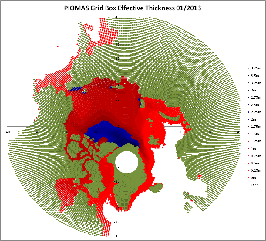
First January 2013.
And now January 2014.
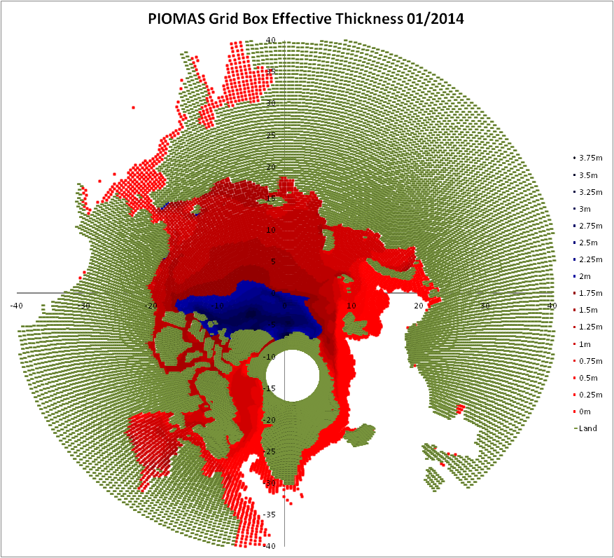
There really isn't much in it from these plots, there's much more ice over 2m thick, but compared to past years there's still barely any ice over 2m thick. For example here's the ice state 20 years ago as modelled in PIOMAS.

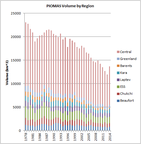
Most of the volume increase is in the Central Arctic, it's a large uptick, but how long will it persist?
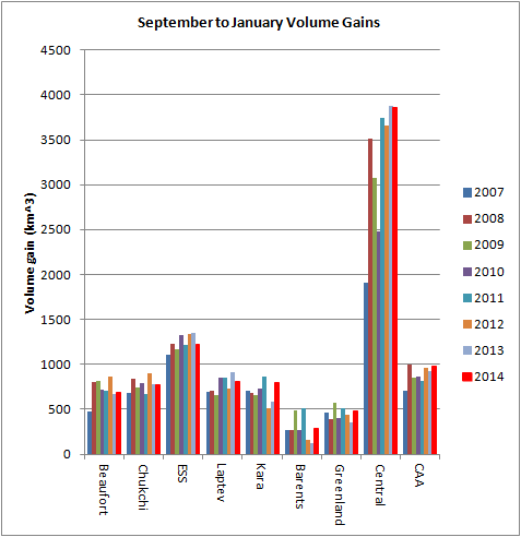
A closer look shows that other regions play a smaller role with increased volume compared to last year at the same time. And it's in the other regions (especially Beaufort to Kara) that much of the summer volume is set and ice conditions set the stage for area/extent losses.

ESS is the East Siberian Sea, CAA is the Canadian Arctic Archipelago.
Volume gains from the preceding September are unremarkable in the context of 2007 onwards.
Breaking down all Arctic volume into contributions from five bands of grid cell effective thickness, and one could be forgiven for thinking it's business as usual.
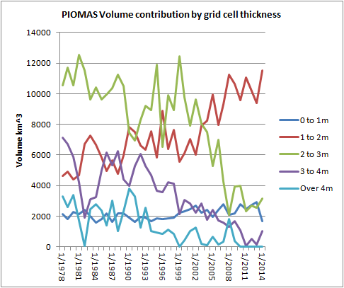
The volume gain hasn't affected the slide from the 2 to 3m band down into the 1 to 2m thick band during this century.
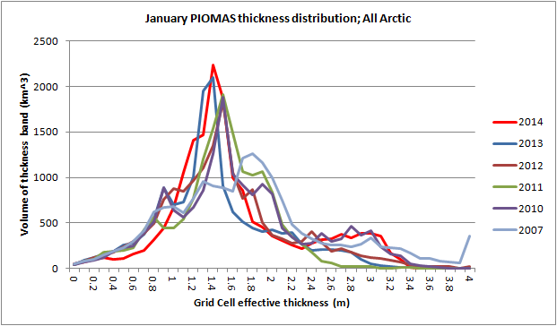
January thickness distribution for the whole PIOMAS domain looks similar to recent years, but check out the hump around 3m thick.
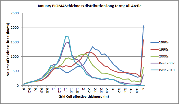
Here's some longer term context. The spikes in the 1980s and 1990s at 4m represent 4m and above, it once contained a lot of volume.
Now for the two 'bell weather' regions outside the Central Arctic, but within the Arctic Ocean.
Beaufort shows the effect of an influx of thick ice from the Central Arctic (hump around 2m), but lies between January 2013 and January 2012. The tall spike is a signature of a lot of FYI thickening thermodynamically.

The East Siberian Sea (ESS) shows an even more prominent mono-modal spike, none of the MYI presence in 2007 is evident, it's still acting like a fully seasonal sea.

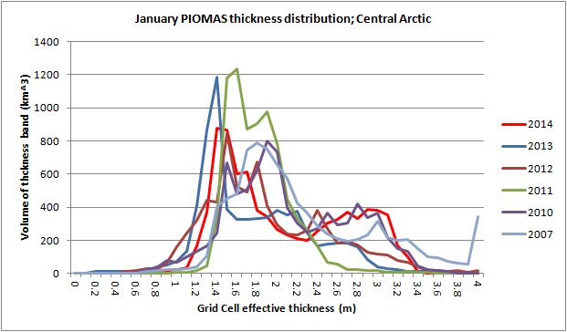
The Central Arctic shows the presence of more thicker ice (~3m) than in other recent years.
Early in January I've said I wasn't expecting a massive loss this year like 2012, I still suspect that without very good melting weather that's unlikely. But aside from the Central Arctic, and that's really confined to the region poleward of Greenland and the CAA, it may not take much for the 2014 season to be rather exciting, as in large losses.
6 comments:
It looks like the 2m+ area for January 2013 is inconsistent with that shown in
http://dosbat.blogspot.com/2013/04/piomas-2013-so-far.html#more
What gives?
There was a difference in definitions in my previous code. The new data is a more understandable demarcation.
In making the maps grid box thicknesses are 'bucketed' into bands of thickness. Previously at say 2m thick that was actually 1.75m to 2.0m. While reworking the code I decided that was a poor way of doing it.
So now the demarcation for say 2m means 2.0m to 2.25m. This done by dividing the thickness by the band (i.e. 0.25m), and taking the integer part of the result as an index of which 'bucket' to put the grid box into.
However it now strikes me that perhaps the blue/red change should be between the 1.75 and 2m thickness bands. I'll change that in the next run of these plots.
Actually I may update these this weekend.
Yeah, that would be nice. I love to be able to just make the visual comparisons. We are such dorks and have such unusual forms of entertainment. :P
I will do so, but I have a problem with my code... groan...
In my old code I could automatically generate named and titled png files. Now I find that in my new code the graph doesn't update. I spent a good chunk of the morning on the problem, but couldn't get to the root of it!
Even if I have to manually save those few I will update tomorrow morning.
O debugging!
Nightvid,
The software bug is sorted now. The images are updated. I have a Google Drive folder with all the images and zips of each decade. See this folder.
Post a Comment