Now that Cryosphere Today's area data (CT Area) are in for yesterday, it's possible to summarise the status for June. The take-home message I read from the data is that a new record is now very unlikely based on past year's behaviour due to the late start to melt, despite other indicators of pack condition (for example the Laptev to N Pole region, link). Posts on the atmospheric status (key to understanding the late melt) and PIOMAS will follow when PIOMAS and NCEP/NCAR updates come in for the month of June.
CT Area is currently below the baseline average period I use (1980 to 1999), but is very high compared to recent years. The last year area on 30 June was this low was 2009, and you have to go back to 2004 before area was regularly above current levels.

This can be better appreciated by the anomalies, which are the differences from the average seasonal cycle as seen in the above graphic as a black line. The anomalies shown below show that while 2013 had a June Cliff, this has now ended and we are into a period of levelling unlike 2011 when anomalies tracked 2007 in a steady decrease. Since 2007 all years have shown an anomaly drop after June through the summer, although in 2010 this drop was delayed by a post-Cliff rise in anomalies. I expect this year to show a drop in anomalies due to the state of the ice enhancing melt rate as compared to the baseline average. However this is not likely to be enough to make a new record, and an interim rise seems to be happening.

The loss through June however has been remarkable given that weather conditions were not conducive to melt and were very anomalous in the context of post 2007 years.
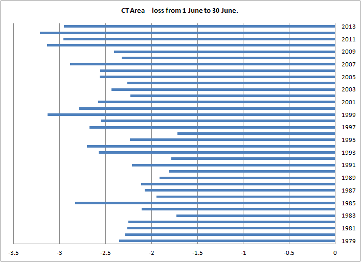
The above graph shows CT Area loss from 1 to 30 June for the CT Area record. June 2013 is seen to join 2010 onwards as a cluster of high loss rate Junes. This might seem favourable for higher loss rates through the rest of the melt season. But there is no trend in loss rates from June 30 to the daily annual minimum over the CT Area record.
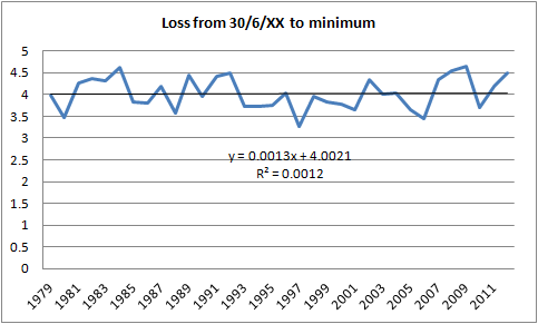
This matches a similar finding by Chris Randles using PIOMAS data for a similar period. There may be more than one reason for this, however it strikes me that losses later in the summer may be limited by available insolation, the ice state for early and late years in the satellite record being similarly degraded by late summer, and thus not being a limiting factor.
The lack of change in CT Area loss from 30 June to minimum (Late Summer Loss) can be applied to this year's area at 30 June to produce a naive prediction. The average Late Summer Loss (4.03M km^2) can be applied to actual 30 June area for each year, and using the standard deviation of Late Summer Losses (0.371M Km^2) a range can be calculated for the prediction. In the following graphic this is visualised.
- The purple plot (mislabelled Series 4 - oops) is actual area at CT Area daily minimum for each year.
- The red plot is the central prediction, calculated simply by applying the average Late Summer Loss from 1979 to 2012 to the actual area at 30 June for the given year.
- The +SD and -SD plots are the central value for a given year with the standard deviation added and subtracted to give the 1 standard deviation ranges for the prediction.
- NB - all the above plots are in 1,000,000 km^2 (1M km^2).
- The bar chart is in units of Sigma, sigma being the standard deviation, and the Sigma Deviation is the deviation from the Central predicted value of the actual area at minimum (Daily CT Area) normalised to the standard deviation. Although I'm using standard deviation, the dataset is too short for me to be sure the distribution is 'normal', so from here onwards the use of standard deviation and sigma is more for convenience that underlying meaning.
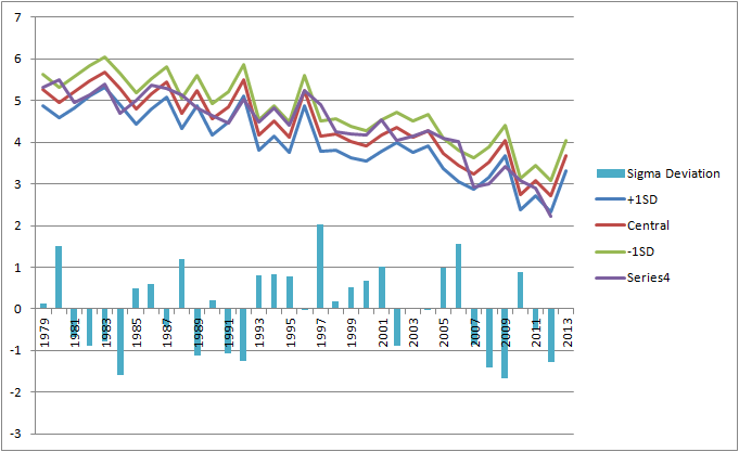
It's worth noting that 2/3 of the predictions are within 1 sigma of the actual value, so although this method is crude it's not worthless. To increase confidence in such a prediction one could merely increase the range, the bar graph above suggests that only something like 1.2 sigma would be needed. However prediction as such isn't my main issue here.
The sigma deviation is useful to examine 2013, and what it would take to make a new record this year and what it would take to beat 2011 (in CT Area 2011 beat the previous record of 2007). In the above graph it can be seen what one gets if one applies the average loss (and +/-sigma bounds) to the CT Area on 30 June 2013. To be specific the prediction for this year is 3.68 M km^2 with bounds (1 sigma) of 3.31 to 4.05M km^2. for the lower bound to meet 2012's record of 2.23M km^2 would require a deviation of -2.90 sigma, for the lower bound to meet 2011's record of 2.90M km^2 would require a deviation of 2.09 sigma.
Now that we know what is needed we can refer to the above graph to get an idea of how likely these are. Technically if the distribution of the deviations is normal then the probability of exceeding 2 sigma would be 4.6%, down to about 0.4% for over 3 sigma. However for the above historical deviation series, in only one instance (2.9%) has a swing as great as that needed for 2013 to beat 2011 occurred, and the deviation needed to beat 2012 has never occurred.
After all this I have reconsidered; I may as well make a prediction...
Using 1.25 sigma, my prediction is:
~75% probability of this year being between 3.22M km^2 and 4.15M km^2.
In other words; approximately between the CT Area daily minima of 2009 (3.42) and 2005 (4.09).
UPDATE - I have narrowed the bounds of my prediction for the purposes of a vote at the Sea Ice Forum, explained here. That prediction is "3.68M to 3.22M km^2, mid point 3.45M km^2" and is a refinement of the above, with lower probability that cannot be calculated as it relies on a heuristic element considering sea ice conditions that were not present for almost all the period post 1979.
UPDATE - I have narrowed the bounds of my prediction for the purposes of a vote at the Sea Ice Forum, explained here. That prediction is "3.68M to 3.22M km^2, mid point 3.45M km^2" and is a refinement of the above, with lower probability that cannot be calculated as it relies on a heuristic element considering sea ice conditions that were not present for almost all the period post 1979.
6 comments:
Do the CT people give a regional breakdown for the historical figures? A lot of this year's "excess" ice over recent years seems to be at low latitudes in (e.g.) Kara/Hudson/Baffin.
One can take the view that these are seasonal seas, will melt out more or less totally and thus be discounted in the regression analysis.
This of course depends on whether extra ice in these seas can have a protective effect on the central pack. For seas like the Laptev and Beaufort, which are continuous with the central basin, then the "pencil sharpening" argument applies - you have to melt through the outer seas before you can start to attack the central basin. For discontinuous regions, then this argument does not apply: it is hard to see how a random floe in the central basin will care about the situation in Hudson and Baffin bays. The Kara sea seems to me to be intermediate in status - although it's technically continuous with the main basin, it has its own separate circulations.
If they do provide local breakdowns for the historical data, could you check whether the regression is improved by discarding any specific regions, and if so how this affects this year's prediction?
Peter,
Good point, as usual. The excess in 'non-shielding' regions and the state of the Laptev/N Pole region could mean I'm totally wrong. It will be interesting to see what the numbers say in September. I don't intend to make another prediction this season, if it becomes apparent something massive is underway I may concede before the minimum.
No, one problem with CT Area is they don't provide regional breakdowns numerically. If they did I'd be on it like a shot.
I wasn't going to make a prediction as such, but after drafting just thought 'what the hell'. It is worth noting that the loss rates from 30 June to minimum (4th fig down) seem to show a slight uptick at the end. I overlooked this deliberately as it's not for all years at the end of the series and the uptick is within variations for the rest of the series. However this could mean that the prediction is biassed high, and that the probability distribution is skewed to the low end of the range.
But even so I'll be very surprised if we see even 2011/2007 being matched this year. And on balance didn't feel the need to look at PIOMAS to commit myself, I'll be staggered if it shows massive loss that undermines this line of reasoning on CT Area data. For better or worse there it is.
Good post, Chris. But as I'm not capable of reasoning like you do, my gut feeling still says we'll end up somewhere between 2012 and 2007/2011.
I feel as if anything is possible, such is the weirdness of this melting season.
Neven,
If this method is wrong it'll be wrong on the low end, i.e. the actual 2013 minimum will be lower. But I've set the bounds to give 76% certainty based on the data.
If I set sigma to 2 then confidence is 97% based on the data, and the lower bound is 2.93, which doesn't quite beat 2011. But having a wider range still means beating 2013 is a long shot.
If we do get a >2 or a 3 sigma deviation this year, that will be telling us something as the magnitude of the June area loss is.
Well, Wipneus has given us a breakdown of the regional differences to 2012 here:
http://forum.arctic-sea-ice.net/index.php/topic,382.msg8577.html#msg8577
Assuming Baffin, Hudson and Kara are irrelevant, that suggests we could adjust the prediction down by ~3/4 of a million or so. That puts us almost spot on 2007, but not as low as 2012, which is where my initial wild-ass guess suggested.
Not unreasonable, but Wipneus' figures should be considered a separate metric. Day 181 is 30/6/13. Wipneus finds Area in 2013 is 266k km^2 ahead of 2012. CT Area as of that date is 977k km^2.
Wipneus finds substantial proportion of the 2013 lead is in Kara and Beaufort, critical 'shielding' regions for the pack.
IIRC Wipneus uses a higher resolution than CT Area seems to. This might explain the difference between Wipneus and CT Area.
Post a Comment