As a result I've been playing around with some toy models based on past behaviour, on the principle that whatever factors are to play a role in what is coming, these factors are already at work. The issue here is not the closeness to observation or the PIOMAS model, but the qualitative form of the output and whether that helps say what will happen in the future.
Is it worth pursuing a simple heuristic model and if so, how can this be improved? Call this Version 1, although there may not be a version 2, depends on people's comments.
The melt season and freeze season are treated as separate periods interlinked by their reliance on initial conditions and passing their final condition on to the next season. Melt season is from annual maximum to annual minimum (daily values), Freeze season is from annual minimum to annual maximum (daily values).
Equations are numbered as per the figure they are derived from.
First the relationship between volume at maximum and volume loss during the season is derived using a scatter plot and the equation of the least squares fit. The fit here is less than ideal, it decreases for larger Volume at Max, and the R2 is only 0.2641. The low R2 demonstrates the problems I've had with the melt season, the freeze season seems to be more dominated by the area at minimum, whereas the melt season is a far more complex period. This is due to the differences in thermodynamic growth in the freeze season and the mix of dynamic and thermodynamic processes in the melt season. The equation form was selected for reasons of visual fit and maximum R2.
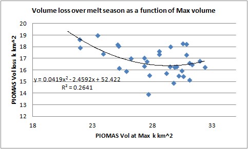
Fig 1. Volume loss in melt season as a function of volume at preceding maximum.
Second the relationship between volume at minimum and volume gain during the melt season is derived using a scatter plot and the equation of the least squares fit. This shows a much better R2, I consider that the general form of the trend line is a reasonable estimate of the underlying form, with weather variability superimposed onto it. The vertical axis label is wrong, it is for the daily maximum not 1 March. The equation form was selected for reason of maximum R2

Fig 2. Volume gain in freeze season as a function of area at preceding minimum.
So that is the melt and freeze seasons calculated, but I now need to transform equation 2 into terms of volume. To do this I convert volume to area so as to provide input for equation 2.
Third the relationship between area and volume at minimum is derived using a scatter plot and the equation of the least squares fit. The equation form was selected to allow fitting to the origin.
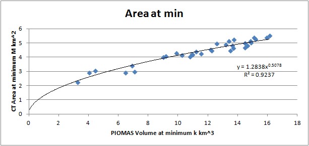
Fig 3. CT Area as a function of PIOMAS volume at daily minimum.
So now I have three equations with which to calculate gain and loss during the freeze and melt seasons. I couple this simply in a spreadsheet where:
Volume at Max = Previous Volume at Min + Previous Volume Gain.
Volume at Min = Current Volume at Max - Current Volume Loss.
Volumes are seeded for the first time slot with PIOMAS volume maximum and minimum for 1980. For current and previous time interval, technically the time interval is a year but it's best not to get to hooked on close correspondence with the real world, what I'm after here is qualitative.
Here is the result.

Fig 4, Output from the toy model.
Obviously the model runs to zero far too fast when compared with observations and PIOMAS. But that is not important, what matters is what is shown qualitatively. The initial drop down is due to adjustment after seeding with actual values not calculated by the model
- Both PIOMAS and the toy model go to zero with a 'bow' to the curve, the rate of change increases with time. This is also apparent in the area output, which shows more of a level start as does CT Area.
- Both PIOMAS and the toy model show volume at minimum departing from volume at maximum, i.e. the annual range increases, from time slot 9 onwards.
- Both PIOMAS and the toy model show a deviation between volume at maximum and minimum as the volume at minimum accelerates towards zero.
Where it gets interesting is that the toy model gets near zero and oscillates. This model does not account for energy gain in the Arctic region due to increasing regions of open water, which would be a factor in reality meaning that indefinite oscillation should not be expected. The equation form was selected because although a logarithmic function would have fitted past behaviour shows no upward or downward trend and no convincing physical justification for either could be seen.
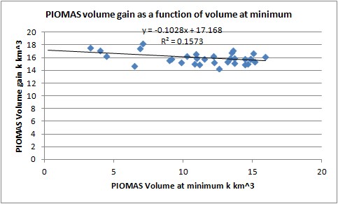
Fig 5, linear relationship between volume gain in freeze season and volume at end of season.
However it is of relevance here that when the toy model is run without equation 2 and 3, but with the linear relationship between melt season and volume gain inserted (fig 5), the output crashes to zero abruptly without oscillation (indeed it goes negative). So is this difference indicative of a long tail caused by the negative thickness/growth feedback in autumn?

Fig 6, model run with the equation in this figure replacing equations 2 and 3. EDIT - now included for completeness.
Does this toy model indicate that we'll see a longish tail as a result of growth thickness feedback causing ice growth in the autumn/winter? I need to think some more about that. But I suspect at present that this does imply a tail (of unknown length) rather than a rapid crash to zero.
One thing I might do to improve the model is to try to factor MYI/FYI ratio into the melt season equation. CT area at the start of June is around 10 million km^2, so the ratio of the minimum area and 10M might be of use as proxy for MYI content. But I'll wait and see what comments there are about this before spending more time on it.
The spreadsheet used to calculate all of this is available here, the source data can be calculated from data in this spreadsheet, sources stated therein on the RawData sheet.
6 comments:
Hi Chris,
This is very similar to what I was trying to do but I was trying to call it a physically based extrapolation.
If you have the volume loss dependant on volume, isn't it logical that the increase in volume loss should be exponential rather than quadratic?
If your model is all based on fits, it seems odd that it is so far out. I am trying to take a look at why but that might take some time.
I decided on modeling the max volume rather than the volume gain. I suggest volume gain in winter doesn't really depend on the minimum it starts from it just approaches a thermodynamic equilibrium. The main components determining the thermodynamic equilibrium, I suggest are GHG level which keep increasing (rather linearly) and upward heat flux.
Is that more physically plausible? if so, the bump in max volume looks odd to me. Is that due to use of quadratic fits or volume at min getting near to 0 or something else?
Crandles,
It's occurred to me that volume levelling out at around 20k km^3 may have a physical basis: the Arctic ocean is around 10M km^2 area of ice at the start of June, when the melt begins within the ocean. If all the ice outside that region, roughly north of 70degN, is thinner adding far less volume, then most of the peak volume comes from (average) 2m thick 10M km^2 area thermodynamically thickened ice with a volume of 20k km^3.
So 20k km^3 represents a floor until winter warming changes the game for thermodynamic thickening.
I've been unable to get to the bottom of why the 'model' drops to zero so much more rapidly than PIOMAS is doing, guestimate - around twice as fast. One factor may be that the curves in figures 1 and 2 are dominated by the recent drop off and may not be giving due weight to the past longer 'lingering' of ice, accelerating progression along the curves faster than has happened in reality.
I've avoided trying a more physical approach as just using fits derived from observations covers all sorts of factors. Although of course I have shaped the behaviour by my choice of what to fit to and the overall partitioning of the year.
A problem I have with introducing base level factors like thermodynamic thickening in terms of the physics is the complexity it introduces. Although maybe I'm wrong in this.
I'm still not convinced I understand why figure two's fit curve has the form it has, i.e. I can't off the top of my head knock together an equation based on the physics that reproduces that curve.
>"I'm still not convinced I understand why figure two's fit curve has the form it has, i.e. I can't off the top of my head knock together an equation based on the physics that reproduces that curve."
Just a guess without much examination:
Is it the case that you have two quadratics? Adding (or subtracting) should just give a quadratic. However I suspect you have a quadratic in max volume and a quadratic in min volume. If they moved together in a 1:1 motion they would still be two quadratics but because they don't move at same speed it is two quadratics in different variables and that can give that bump.
I expect that using exponential rather than quadratic would give much better fit to the data.
Crandles,
As it says in the post, a quadratic was chosen to maximise R2. An exponential gives:
Y=20.36*Exp(-0.055X)
Where X is the previous year's minimum area.
This has an R2 of 0.5622, and is closer to linear (as can be appreciated from the 0.055), where a linear an R2 of 0.5752.
However having been pondering the matter I cannot see a reason to expect a strongly non linear ice growth in response to area of preceding season's. Geometry suggests this should be linear. The open water at the end of the season is merely replaced by new ice of thermodynamic equilibrium thickness ~2m.
When I put the linear equation into the toy I get a rapid crash to zero, with a negligible tail due to constraining minimum volume to > zero. Because the quadratic ice growth counters the losses more actively as volume/area decreases, this extends the crash to minimum until year 21 or so, in the case of a linear ice growth response the ice crashes out rapidly to zero by year 17.
This makes me happier because a fast crash would be more exciting than a drawn out tail.
I'll blog on this tomorrow.
I'm pondering throwing this problem at a very smart person. I never got round to pursuing this further. Frankly at the moment I'm not able to move this forward.
Post a Comment